
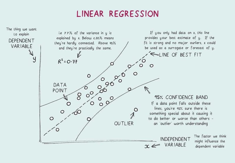
Linear regression is a supervised machine learning technique where we train a ML algorithm on labeled datasets. Basically, it is a statistical model that identifies the relationship between independent and dependent variables. Here, we predict the target value based on input variables. The linear regression model finds the best-fit line for our model.
The hypothesis for linear regression is defined as:
y = m*x + c
y: output variable
m : gradient
x : input variable
c : intercept
When we train the model, it fits the best-fit line to predict the value of y for a given value of x, by determining the values of m and c. Once we find the optimal values of m and c, we obtain the best-fit line, enabling us to use our model for prediction.
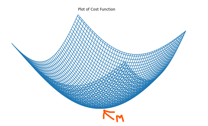
Cost Function:
The cost function quantifies the error between predicted and true values, aiming to minimize this difference. Mathematically, it is represented as the root mean square error (RMSE) between predicted and true values:
cost function = sqrt((∑(pred(i) – y(i))^2) / n)
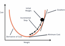
Gradient Descent:
In gradient descent, the model strives to minimize the cost function by iteratively updating the parameters m and c. Initially, these parameters are randomly initialized and updated iteratively until optimal values are found. Through this process, the model achieves the minimum cost function with optimal values of m and c.
Math Behind Machine Learning Algorithm :
Forward Propagation :
assuming the hypothesis y = m * x + c
differentiating cost function :
∂(Cost Function) / ∂(m) = (1 / n) * ∑((pred(i) – y(i)) * x(i))
∂(Cost Function) / ∂(c) = (1 / n) * ∑(pred(i) – y(i))
parameter updation :
m’ = m – α * ∂(Cost Function) / ∂(m)
c’ = c – α * ∂(Cost Function) / ∂(c)
Here, α (alpha) represents the learning rate, determining the step size in the parameter space during optimization.
Linear Regression Algorithm :
import numpy as np
import matplotlib.pyplot as plt
# Load the dataset
data = pd.read_csv(“data_for_lr.csv“)
# Split data into training and testing sets
train_input = np.array(data.x[:500]).reshape(500,1)
train_output = np.array(data.y[:500]).reshape(500,1)
test_input = np.array(data.x[500:700]).reshape(199,1)
test_output = np.array(data.y[500:699]).reshape(199,1)
def forwardPropagation(train_input, parameters):
m = parameters[‘m‘]
c = parameters[‘c‘]
prediction = np.multiply(m, train_input) + c
return prediction
# Cost function to evaluate the error between predictions and actual values
def costFunction(prediction, train_output):
cost = np.mean((train_output – prediction) ** 2) * 0.5
return cost
# Backward propagation function to compute derivatives
def backwardPropagation(train_input, train_output, prediction):
derivatives = dict()
df = prediction – train_output
dm = np.mean(np.multiply(df, train_input))
dc = np.mean(df)
derivatives[‘dm‘] = dm
derivatives[‘dc‘] = dc
return derivatives
# Function to update parameters using gradient descent
def updateParameters(parameters, derivatives, learning_rate):
parameters[‘m‘] = parameters[‘m‘] – learning_rate * derivatives[‘dm‘]
parameters[‘c‘] = parameters[‘c‘] – learning_rate * derivatives[‘dc‘]
return parameters
def train(train_input, train_output, learning_rate, iters):
# Initialize parameters with random values
parameters = dict()
parameters[‘m‘] = np.random.uniform(0, 1)
parameters[‘c‘] = np.random.uniform(0, 1)
# List to store loss values for each iteration
loss = list()
# Iterate over specified number of iterations
for i in range(iters):
# Perform forward propagation
prediction = forwardPropagation(train_input, parameters)
# Compute cost
cost = costFunction(prediction, train_output)
loss.append(cost)
print(f‘Iterations : {i+1}, loss : {cost}‘)
# Plot training data and predictions
plt.figure()
plt.plot(train_input, train_output, ‘+‘, label=‘Original‘)
plt.plot(train_input, prediction, ‘–‘, label=‘Training‘)
plt.legend()
plt.show()
# Perform backward propagation
derivatives = backwardPropagation(train_input, train_output, prediction)
# Update parameters
parameters = updateParameters(parameters, derivatives, learning_rate)
return parameters, loss
# Perform training
parameters, loss = train(train_input, train_output, 0.0001, 10)
during training
y_predict = test_input * parameters[‘m‘] + parameters[‘c‘]
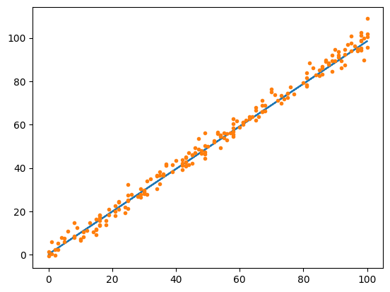
# Plot predicted values against test data
plt.plot(test_input, y_predict, ‘–‘)
plt.plot(test_input, test_output, ‘.‘)
plt.show()
Linear regression is commonly used for training, and its subsequent prediction is facilitated by determining the best-fit line. This line indicates that we have found values close enough to the input data. However, linear regression has limitations; it struggles to handle outliers effectively, and categorical data encoding is required each time, among other challenges.

